Bezier Curves

A Bézier curve is a method for representing curves popularized by the French engineer Pierre Bézier in the 1960's. Bézier used the curves in the design of automobiles. The curves are still popular today in drawing and animation applications because they offer an intuitive control over curve shape. Bézier curves can also be approximated very easily using a recursive algorithm developed by another Frenchman, Paul de Casteljau. You are going to create a program that allows users to draw a Bézier curve.

Setup

Create a directory assignment6 under assignments in your cs170 directory. All code for the assignment should be stored in this directory.

cd ~/cs170/assignments
mkdir assignment6 
cd assignment6

Details

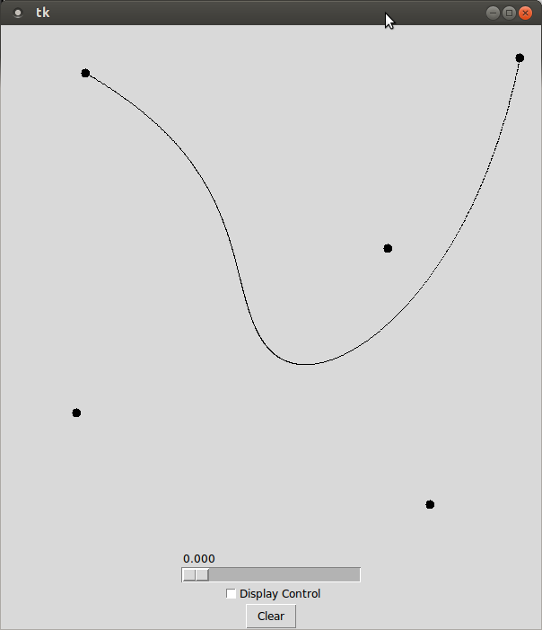
The program should display a window that adds small circles whereever the mouse is clicked. Each circle in the window is a control point for a Bézier curve. Each time a control point is added the display should redraw the Bézier curve to include the new control point.

The de Casteljau algorithm can be used to generate a single point that exists on the bezier curve. It is a recursive algorithm takes two parameters: A list of control points and a floating point value \(t\) in the range [0, 1]. The de Casteljau algorithm returns the point that is \(t \%\) along the bezier curve. To draw the entire curve, you will compute a fixed amount of evenly spaced points on the curve (which are computed by varying the value of \(t\) provided to the algorithm). You will then connect consecutive points along the curve using straight lines. By default, your program does not need to draw the control structure.

The de Casteljau algorithm can be expressed recursively using the following equations:

\[ \begin{eqnarray} de\_casteljau([ p_1 ], t) &=& p1\\ de\_casteljau([ p_1, \ldots, p_n ], t) &=& de\_casteljau([ linear\_interpolate(p_1, p_2, t), linear\_interpolate(p_2, p_3, t), \ldots, linear\_interpolate(p_{n-1}, p_{n}, t) ], t) \end{eqnarray} \]

Where t is the is a floating point value in the range [0, 1] representing the parametric distance, linear_interpolate finds the point at the specified parametric distance between two points, and the square brackets specify a list of points.

Pseudo Code

Linear Interpolation

We have not talked about linear interpolation this semester, although you have indirectly been using it in a handful of programs. You are given two real numbers \(x_1\) and \(x_2\), and a parametric distance \(t\) in the range [0, 1]. You need to find the real value \(x_3\) that is \(t \%\) between \(x_1\) and \(x_2\).

For Monday, Feb. 24^th, I want you to turn in (on paper!) pseudo code for the linear interpolation function, with 2 test cases that demonstrate that you understand how the code should operate.

Submission

You are required to submit a tar file to http://inquire.roanoke.edu/. On inquire, there is a link for Assignment 6. You can create a tar file by issuing the following commands:

cd ~/cs170/assignments
tar czvf assignment6.tgz assignment6/

"Hacker" Prompt

1. Movable Control Points: Add the ability to modify a Bézier curve after it has been drawn by dragging its control points. When the user is dragging a control point, the Bézier curve should be redrawn every time the mouse drag call-back function is called.

2. de Casteljau Slider: One of the interesting things about the de Casteljau algorithm is the "recursive descent" that occurs in order to find a particular point on the true curve. While you likely were able to create the Bézier without having a good visualization of how it works. The actual process that is going on, however, is pretty cool looking.

   Create an additional panel to your tk window, that has a tk.Checkbutton and a tk.Scale widget. If the check button is selected, you should display the control structure of the Bézier curve. You should use the slider to pick the parametric distance t. This control structure should display how the t^th point of the curve was generated.