CPSC120 - Activity 11

Interpolate

Interpolating is the process of estimating an unknown value by using known values. In linear interpolation, you find a value some fraction of the distance along the line between two values. For example, the value halfway between 0 and 10 is 5. And the value one-quarter of the way between 0 and 10 is 2.5. You can also interpolate between two 2D-points by interpolating the x and y coordinates separately.

Details

Create a Python program that defines the function interpolate(start: float, end: float, fraction: float) -> float that linearly interpolates between two values. Use this equation to interpolate between any two values:

\(between = start \cdot (1 - fraction) + end \cdot fraction\)

Test Cases

import test

def main() -> None:
    test.equal(interpolate(0.0, 1.0, 0.5), 0.5)
    # Add more test cases here.
    return None

main()

Tweening

In traditional hand-drawn animation, senior animators would draw the most critical frames of an animation sequence, the keyframes. Then the junior animators would be responsible for filling in all of the in-between frames. Creating the between frames in computer animation is still called tweening, although it is performed automatically by computers.

Details

Create a Python program that defines the function tween(start_x: float, start_y: float, end_x: float, end_y: float, frames: int) -> None that animates a circle moving between two keyframes. The circle should start at the point (start_x, start_y) and move in a straight line to the point (end_x, end_y). The animation should be frames long.

Example

import graphics

def main() -> None:
    width: float
    x: float
    graphics.double_buffer()
    width = graphics.screen_width()
    x = width / 2.0 - 25.0
    for i in range(0, 3, 1):
        tween(x, 0.0, -x, 0.0, 120)
        tween(-x, 0.0, x, 0.0, 120)
    return None

main()

Hint

The circle will be moving in a straight line between the start and endpoints, so its position will be linearly interpolated between the start and endpoints.
Copy the interpolate function into this program to make writing the tween function easier.
Remember that animation requires a loop that clears, draws, updates, and waits.
When drawing the circle, calculate its x coordinate by interpolating the keyframes’ x coordinates. And calculate the y coordinate by interpolating the keyframe’s y coordinates.
The interpolation fraction should be the current fraction of the animation frames. So the first frame is 0. The middle frame is 0.5. The last frame is 1.0. Calculate the fraction by dividing the current frame number by the total number of frames.

Challenge

Linear interpolation creates artificial-looking animations because objects can instantaneously accelerate. Smoother, more realistic animations can be created by modifying the interpolation fraction. A common modification is a sigmoid function. Modify the tween function so that it uses a sigmoid function to smooth out the animation.

Move

Creating a program where the robot car navigates along a particular path is difficult because the correct speed and duration needed to produce a specific movement are very difficult to determine. Writing navigation code can be significantly simplified by using functions to build complex movements out of simpler ones.

Details

Create a Python program that defines the functions forward() -> None left() -> None and right() -> None that move and turn the car. The forward function should move the car forward one square of the ground grid. The left and right functions should turn the car 90 degrees, in-place, left and right. These functions should assume that the car is not moving when the function is called and should stop call car movement before finishing. These functions do not need to be exact. In fact, the randomness of the simulation makes that impossible for now.

Example

import robotics

def main() -> None:
    robotics.add_ground()
    robotics.add_car()
    robotics.wait(1000)
    right()
    forward()
    left()
    forward()
    return None

main()

Hint

To move the car forward, set both wheels’ speed to a positive value, wait for a duration, and then stop the wheels.
To turn the car, set the wheel speeds to positive and negative values, wait for a duration, the stop the wheels.
You will need to experiment with different combinations of wheel speed and duration to move the correct distance.
The slower the car moves, the less impact the simulation randomness will have on the function.

Maze

A classic robotics problem is maze navigation. Efficiently navigating a unique maze requires the ability to sense and remember the maze structure. Creating a program to follow a predetermined path through the maze is easier.

Details

Create a Python program that defines the functions add_maze() -> None that creates a maze for the robot car to navigate.

Example

import robotics

def main() -> None
    robotics.add_ground(100.0, 100.0, 15, 15)
    robotics.add_car()
    add_maze()
    return None

main()

Hint

Create a maze by adding boxes with the same height, width, and depth as the ground grid cells.
The default ground grid is 100 x 100 units with 15 x 15 squares. So a single cell is 100 / 15 units on a side.
Creating the maze is much easier if you have a function. Create the function `add_wall(row: int, col: int) -> that adds a block given the row and column of a cell.
Then the add_maze function can repeatedly call the add_wall function.

Challenge

Use the forward, left, and right functions to navigate the maze you created.

Bivariate Plotting

By plotting a single attribute in a dataset, we can get an idea of typical values and spread. But to find unusual things in our data, we need to explore the relationship between different attributes. An excellent place to start is by creating a 2D plot of two attributes.

Details

Create a Python program that defines the function plot_bivariate(col1: int, col2: int) -> None that plots two different columns of a spreadsheet. For each row in the spreadsheet, draw a point. The point’s x-coordinate is the value in col1, and the y-coordinate is the value in col2.

Example

import spreadsheet
import plot

def main() -> None:
    spreadsheet.load("https://www.humblepython.com/static/editor/data/AddHealthWaveI.csv")
    plot_bivariate(1, 3)
    return None

main()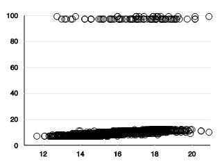

Bivariate

Hint

Like the univariate plotting that you previously wrote, you need a for loop that iterates over the rows of the spreadsheet.
For each row, use the spreadsheet.get function to get the x and y coordiantes of a point to draw.
The x-coordinate is the value from column col1 and the y-coordinate is the value from column col2 in the current row.
Use the plot.draw_point function to draw each point.

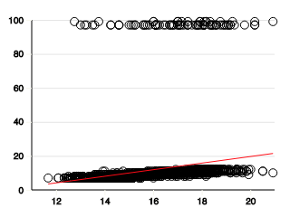
Regression

Plotting two columns in a dataset lets us see the relationship between two attributes. Still, sometimes we need to quantify the relationship. Regression is the process of estimating the relationship between two attributes. Linear regression models this relationship using a line. A common way of computing this line is the least-squares method, where we compute the slope of the line that most closely fits the data.

Details

Create a Python program that defines the function compute_least_squares(col1: int, col2: int) -> float that uses least squares to compute the line’s slope that fits the points of two columns of a spreadsheet. Use this equation to calculate the slope:

\[m = \frac{\sum_{i=1}^{n} (x_i - \bar{x}) (y_i - \bar{y})}{\sum_{i=1}^{n} (x_i - \bar{x}) (x_i - \bar{x})}\]

The values x_i and y_i are the i^th values in a columns 1 and 2. The values \(\bar{x}\) and \(\bar{y}\) are the mean of the values in columns 1 and 2. And the value n is the number of values in a column.

Test

import spreadsheet
import test

def main() -> None:
    spreadsheet.load("https://www.humblepython.com/static/editor/data/AddHealthWaveI.csv")
    test.equal(compute_least_squares(1, 3), 1.938394558267123)
    return None

main()

Hint

Before computing the sums in the slope equation, you will need to calculate the two columns’ mean.
Copy the mean code you previously wrote into this program, but make it a function. That way, you can call the function twice, once for each of the two columns.
To compute the slope, you will need two accumulator variables, one for each of the sums.
You only need one loop, though. This one loop can compute both sums by update both accumulators each iteration of the loop.

Challenge

Plot the least squares line by drawing a line through the point \((\bar{x}, \bar{y})\) using the plot.draw_line function.

Least Squares